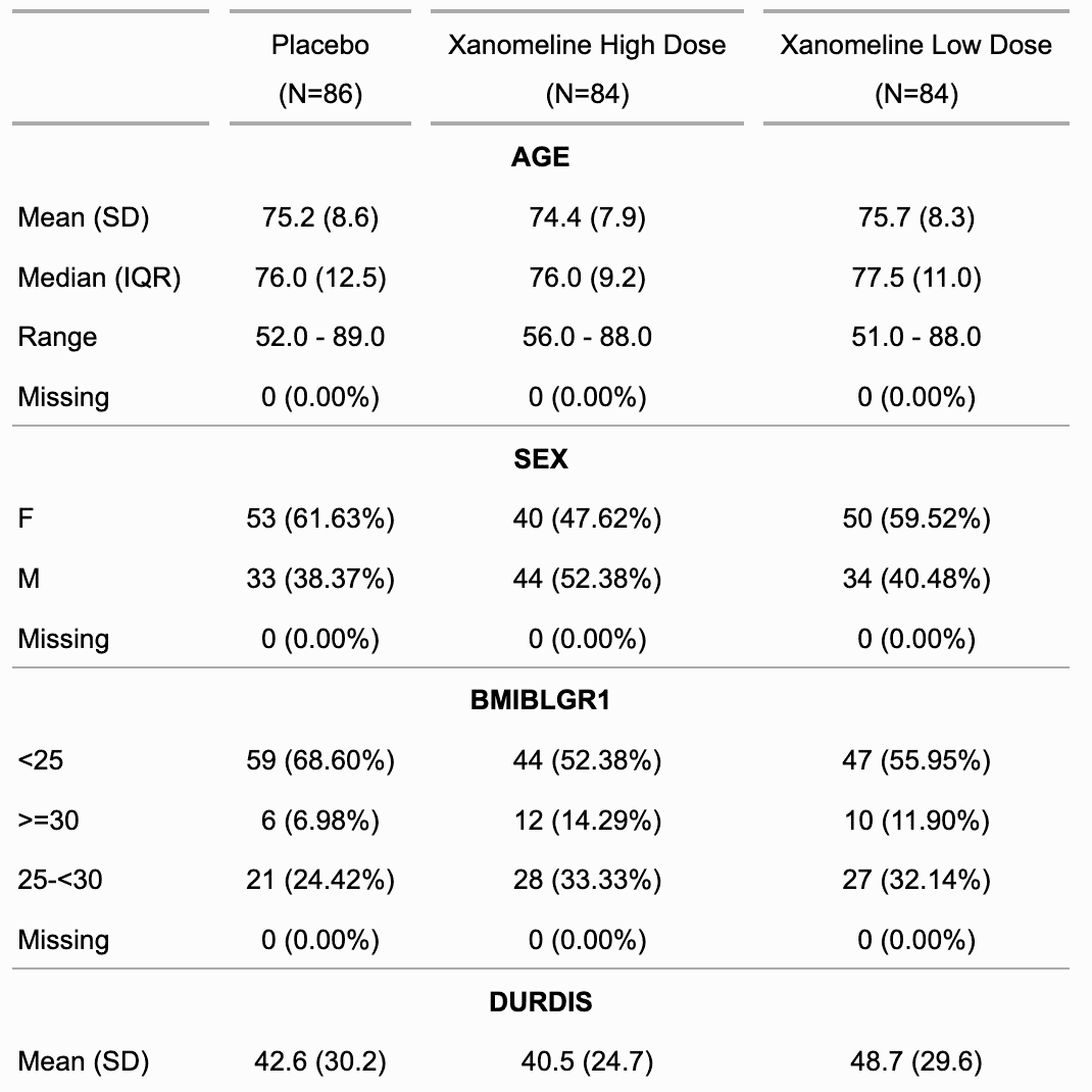
It performs a univariate statistical analysis of a dataset
by group and formats the results so that they can be used with
the tabulator() function or directly with as_flextable.
Arguments
- x
dataset
- by
columns names to be used as grouping columns
- overall_label
label to use as overall label
- num_stats
available statistics for numerical columns to show, available options are "mean_sd", "median_iqr" and "range".
- hide_null_na
if TRUE (default), NA counts will not be shown when 0.
- use_labels
Logical; if TRUE, any column labels or value labels present in the dataset will be used for display purposes. Defaults to TRUE.
Examples
z <- summarizor(CO2[-c(1, 4)],
by = "Treatment",
overall_label = "Overall"
)
ft_1 <- as_flextable(z)
ft_1
nonchilled
(N=40)
chilled
(N=42)
Overall
(N=82)
Plant
Qn1
5 (12.5%)
0 (0.0%)
5 (6.1%)
Qn2
7 (17.5%)
0 (0.0%)
7 (8.5%)
Qn3
7 (17.5%)
0 (0.0%)
7 (8.5%)
Qc1
0 (0.0%)
7 (16.7%)
7 (8.5%)
Qc3
0 (0.0%)
7 (16.7%)
7 (8.5%)
Qc2
0 (0.0%)
7 (16.7%)
7 (8.5%)
Mn3
7 (17.5%)
0 (0.0%)
7 (8.5%)
Mn2
7 (17.5%)
0 (0.0%)
7 (8.5%)
Mn1
7 (17.5%)
0 (0.0%)
7 (8.5%)
Mc2
0 (0.0%)
7 (16.7%)
7 (8.5%)
Mc3
0 (0.0%)
7 (16.7%)
7 (8.5%)
Mc1
0 (0.0%)
7 (16.7%)
7 (8.5%)
Type
Quebec
19 (47.5%)
21 (50.0%)
40 (48.8%)
Mississippi
21 (52.5%)
21 (50.0%)
42 (51.2%)
conc
Mean (SD)
445.6 (299.9)
435.0 (297.7)
440.2 (297.0)
Median (IQR)
350.0 (500.0)
350.0 (500.0)
350.0 (500.0)
Range
95.0 - 1,000.0
95.0 - 1,000.0
95.0 - 1,000.0
uptake
Mean (SD)
30.8 (9.6)
23.8 (10.9)
27.2 (10.8)
Median (IQR)
31.3 (12.3)
19.7 (20.4)
28.3 (18.8)
Range
10.6 - 45.5
7.7 - 42.4
7.7 - 45.5
ft_2 <- as_flextable(z, sep_w = 0, spread_first_col = TRUE)
ft_2
nonchilled
(N=40)
chilled
(N=42)
Overall
(N=82)
Plant
Qn1
5 (12.5%)
0 (0.0%)
5 (6.1%)
Qn2
7 (17.5%)
0 (0.0%)
7 (8.5%)
Qn3
7 (17.5%)
0 (0.0%)
7 (8.5%)
Qc1
0 (0.0%)
7 (16.7%)
7 (8.5%)
Qc3
0 (0.0%)
7 (16.7%)
7 (8.5%)
Qc2
0 (0.0%)
7 (16.7%)
7 (8.5%)
Mn3
7 (17.5%)
0 (0.0%)
7 (8.5%)
Mn2
7 (17.5%)
0 (0.0%)
7 (8.5%)
Mn1
7 (17.5%)
0 (0.0%)
7 (8.5%)
Mc2
0 (0.0%)
7 (16.7%)
7 (8.5%)
Mc3
0 (0.0%)
7 (16.7%)
7 (8.5%)
Mc1
0 (0.0%)
7 (16.7%)
7 (8.5%)
Type
Quebec
19 (47.5%)
21 (50.0%)
40 (48.8%)
Mississippi
21 (52.5%)
21 (50.0%)
42 (51.2%)
conc
Mean (SD)
445.6 (299.9)
435.0 (297.7)
440.2 (297.0)
Median (IQR)
350.0 (500.0)
350.0 (500.0)
350.0 (500.0)
Range
95.0 - 1,000.0
95.0 - 1,000.0
95.0 - 1,000.0
uptake
Mean (SD)
30.8 (9.6)
23.8 (10.9)
27.2 (10.8)
Median (IQR)
31.3 (12.3)
19.7 (20.4)
28.3 (18.8)
Range
10.6 - 45.5
7.7 - 42.4
7.7 - 45.5
z <- summarizor(CO2[-c(1, 4)])
ft_3 <- as_flextable(z, sep_w = 0, spread_first_col = TRUE)
ft_3
Statistic
(N=82)
Plant
Qn1
5 (6.1%)
Qn2
7 (8.5%)
Qn3
7 (8.5%)
Qc1
7 (8.5%)
Qc3
7 (8.5%)
Qc2
7 (8.5%)
Mn3
7 (8.5%)
Mn2
7 (8.5%)
Mn1
7 (8.5%)
Mc2
7 (8.5%)
Mc3
7 (8.5%)
Mc1
7 (8.5%)
Type
Quebec
40 (48.8%)
Mississippi
42 (51.2%)
Treatment
nonchilled
40 (48.8%)
chilled
42 (51.2%)
conc
Mean (SD)
440.2 (297.0)
Median (IQR)
350.0 (500.0)
Range
95.0 - 1,000.0
uptake
Mean (SD)
27.2 (10.8)
Median (IQR)
28.3 (18.8)
Range
7.7 - 45.5