Tabulation of aggregations

It tabulates a data.frame representing an aggregation which is then transformed as a flextable with as_flextable. The function allows to define any display with the syntax of flextable in a table whose layout is showing dimensions of the aggregation across rows and columns. tabulator illustration

Usage

tabulator(
  x,
  rows,
  columns,
  datasup_first = NULL,
  datasup_last = NULL,
  hidden_data = NULL,
  row_compose = list(),
  ...
)

# S3 method for class 'tabulator'
summary(object, ...)

Arguments

x: an aggregated data.frame
rows: column names to use in rows dimensions
columns: column names to use in columns dimensions
datasup_first: additional data that will be merged with table and placed after the columns presenting the row dimensions.
datasup_last: additional data that will be merged with table and placed at the end of the table.
hidden_data: additional data that will be merged with table, the columns are not presented but can be used with compose() or mk_par() function.
row_compose: a list of call to as_paragraph() - these calls will be applied to the row dimensions (the name is used to target the displayed column).
...: named arguments calling function as_paragraph(). The names are used as labels and the values are evaluated when the flextable is created.
object: an object returned by function tabulator().

Value

an object of class tabulator.

Methods (by generic)

summary(tabulator): call summary() to get a data.frame describing mappings between variables and their names in the flextable. This data.frame contains a column named col_keys where are stored the names that can be used for further selections.

Note

This is very first version of the function; be aware it can evolve or change.

Examples

if (FALSE) { # \dontrun{
set_flextable_defaults(digits = 2, border.color = "gray")

library(data.table)
# example 1 ----
if (require("stats")) {
  dat <- aggregate(breaks ~ wool + tension,
    data = warpbreaks, mean
  )

  cft_1 <- tabulator(
    x = dat, rows = "wool",
    columns = "tension",
    `mean` = as_paragraph(as_chunk(breaks)),
    `(N)` = as_paragraph(as_chunk(length(breaks), formatter = fmt_int))
  )

  ft_1 <- as_flextable(cft_1)
  ft_1
}

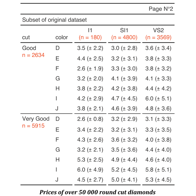
# example 2 ----
if (require("ggplot2")) {
  multi_fun <- function(x) {
    list(mean = mean(x), sd = sd(x))
  }

  dat <- as.data.table(ggplot2::diamonds)
  dat <- dat[cut %in% c("Fair", "Good", "Very Good")]

  dat <- dat[, unlist(lapply(.SD, multi_fun),
    recursive = FALSE
  ),
  .SDcols = c("z", "y"),
  by = c("cut", "color")
  ]

  tab_2 <- tabulator(
    x = dat, rows = "color",
    columns = "cut",
    `z stats` = as_paragraph(as_chunk(fmt_avg_dev(z.mean, z.sd, digit2 = 2))),
    `y stats` = as_paragraph(as_chunk(fmt_avg_dev(y.mean, y.sd, digit2 = 2)))
  )
  ft_2 <- as_flextable(tab_2)
  ft_2 <- autofit(x = ft_2, add_w = .05)
  ft_2
}

# example 3 ----
# data.table version
dat <- melt(as.data.table(iris),
  id.vars = "Species",
  variable.name = "name", value.name = "value"
)
dat <- dat[,
  list(
    avg = mean(value, na.rm = TRUE),
    sd = sd(value, na.rm = TRUE)
  ),
  by = c("Species", "name")
]
# dplyr version
# library(dplyr)
# dat <- iris %>%
#   pivot_longer(cols = -c(Species)) %>%
#   group_by(Species, name) %>%
#   summarise(avg = mean(value, na.rm = TRUE),
#   sd = sd(value, na.rm = TRUE),
#   .groups = "drop")

tab_3 <- tabulator(
  x = dat, rows = c("Species"),
  columns = "name",
  `mean (sd)` = as_paragraph(
    as_chunk(avg),
    " (", as_chunk(sd), ")"
  )
)
ft_3 <- as_flextable(tab_3)
ft_3

init_flextable_defaults()
} # }